PolyMix-2
Here is PolyMix-2 at a glance.
Workload Name: PolyMix-2 Polygraph Version: 2.2.9 Configuration: workloads/polymix-2.pg Workload Parameters: peak request rate and
proxy environmentResults: available Synopsis: workload designed specifically for the second bake-off
Table of Contents
1. Objectives
2. Load generation
3. Traffic model
3.1 constant working set size
4. Simulating WAN environment
4.1 Low-level simulation
4.2 High-level simulation
4.3 The choice
5. IP allocation
5.1 Allocation scheme
5.2 Number of clients and servers
5.3 Configuration example
5.4 Other provisions
1. Objectives
PolyMix-2 is based on our experience with using PolyMix-1 and DataComm-1 during the first bake-off and other tests. We are trying to eliminate some of the known problems of the old workloads and add new features. The ultimate goal is, of course, getting our model closer to the real worlds. Here is a list of most important objectives:
- remove unintended run-duration-dependent variations in workload characteristics (e.g., steadily decreasing memory hit ratio)
- check whether a proxy under test is in a ``steady state''
- remove 1:1 mapping between servers and clients
- more realistic proxy load modeling
- better response size distributions
- model variety of request types (e.g. "Reload" and "IMS" requests)
- model inter-object dependencies
- model object life cycle
- model WAN environment
2. Load generation
PolyMix-2 introduces a new model for simulating proxy load. Previous workloads supported ``best-effort'' and ``constant'' request rate models. Both models represented only a short segment of load pattern seen on most real proxies. The latter had a few unfortunate side-effects, including extremely sharp increase in load and absence of ``relaxation'' time. We were also not satisfied with the necessity to run many experiments for performance-versus-load analysis.
Here is a simple diagram showing a four day trace of proxy load. Note the 24 hour period of the pattern.
Despite the temptation, we do not want to run three-four day tests. We want to take the most interesting part of a periodic load pattern and simulate it. The dark area on the trace above represents the spot we are interested in. We also do not want to have a 14 hour long idle period (the area between two humps). We shorten the idle period to 2 hours. The result is shown below, with labels representing time since the start of a run.
Note the steady load increase during the first hour of an experiment. We do not want to start immediately with peak request rate. The load pattern represents two busy days in life of a proxy, with ``first morning'' and ``last night'' periods cut off:
Simulation
HoursActivity 00 - 01 The load is increased during the first hour to reach its peak level. 01 - 05 The period of peak ``daily'' load. 05 - 06 The load steadily goes down, reaching a period of relatively low load. 06 - 08 The ``idle'' period with load level around 10% of the peak request rate. 08 - 09 The load is increased to reach its peak level again. 09 - 13 The second period of peak ``daily'' load. 13 - 14 The load steadily goes down to zero. As usual, Polygraph parameters allow to change the absolute numbers discussed here, preserving the load curve shape. For example, the idle period can be shorten to, say, 30 minutes if a proxy is known to do nothing during its idle time.
The load pattern has several nice properties.
Comparing the performance on two humps tells us if a proxy has not reached a steady state.
Periods of high load are long enough to gether comprehensive statistics about a proxy under peak load (the interesting case).
Steady change in load levels on hump sides allows to build performance-versus-load graphs.
The idle period allows a proxy to do its regular off-line activities like lazy garbage collection.
The presence of both idle and busy periods allows us to determine which ``deficiencies' of a proxy are load dependent.
A user does not have to run the entire 14 hour test to find out the sustained peak request rate a proxy can support. If a user is confident that a proxy is in a steady state, simulating just the first hump is enough. At the bake-off, we know that a proxy may not be in a steady state right after the fill.
3. Traffic model
3.1 constant working set size
One of the biggest challenges posed by long tests is providing a ``stable'' workload. We want a proxy to reach its steady state of operation if such a state exists. If the workload itself changes during the entire run, then a proxy may never reach steady state.
Let's define working set as the set of all objects that have non-zero probability of access at a given time. To simulate cachable misses, a benchmark needs to introduce new cachable objects into the working set (a so called ``fill'' stream). Thus, the working set size grows during the duration of an experiment. Growing working set implies changing access probabilities for each URL in the set because the sum of the probabilities is equal to 100%. Changing probabilities clearly violate ``stable workload'' requirement.
To avoid problems associated with the growing working set, we have to artificially limit its size. Technically, enforcing the limit is easy: We simply instruct Polygraph not to request objects that were introduced into the working set ``some time'' ago. The problem is to select the size that is
- fair to all products under test
- small enough to get steady state conditions early in the test
- large enough to require proxies to cache realistic amount of traffic
We address the first challenge by specifying the size of the working set based on time rather than number of objects or their total size. We configure Polygraph to freeze working set size after the first X hours of the experiment. In other words, the number of objects a proxy processed during the first X hours becomes the size of the working set for that proxy. This approach makes the limit independent from cache capacity or proxy speed.
The second requirement is easy to satisfy (in isolation). For example, the X value of one hour would be perfect because it would achieve steady state conditions before the first peak rate phase.
The third challenge is impossible to meet because the duration of the test is too short. Even if we set working set size to 14 hours, that is still not large enough. A real proxy should cache at least two-three days worth of traffic. The following two approaches can be used to address the problem.
First, we can make the duration of the experiment longer. Second, we can reuse objects that were cached during the filling-the-cache run. Unfortunately, both solutions are not suitable for our benchmarking environment. Thus, our only hope is that whoever interprets the results will keep cache capacity in mind and will ignore proxy configurations that could not cache a few days of traffic under the advertised request rate. To assist the reader, we will compute and publish the amount of data a cache can keep (e.g., ``proxy A can keep 1 day worth of PolyMix-like traffic''). For the bake-off, the latter may encourage vendors to bring proxy configurations that ``make sense'' given the request rates advertised by a vendor.
In short, we want to keep the value of X as large as possible but no larger than 6 hours to get steady state conditions before the idle phase and the second peak phase.
The proposed value for X is 4 hours. This value gives us about an hour of steady state conditions during the first peak phase so we have something to compare with the second peak phase. Note that as far as set size is concerned, the first 4 hours are approximately equivalent to 3.5 hours of peak request rate load.
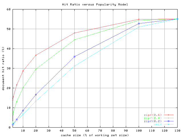
Clearly, the working set size among with the popularity model will affect [memory] hit ratios. Here are the approximate hit ratio results based on a simulated cache with an LRU replacement policy.
Cache Size
(% of working set size)Hit Ratio(%) Unif Zipf(0.2) Zipf(0.4) Zipf(0.6) 2.0 1.3 1.4 1.6 13.7 2.5 1.7 1.9 7.8 15.5 5.0 3.4 4.0 13.1 21.6 10.0 6.7 8.5 20.2 28.7 20.0 13.3 16.7 29.5 36.7 50.0 31.1 36.0 44.5 48.0 100.0 51.0 52.8 54.4 54.9 130.0 55.0 55.0 55.0 55.0
The results for the first and last lines were obtained using commands similar to these.
pop_test --cache_size  1MB \
    --pop_model unif
pop_test --cache_size 50MB \
    --pop_model zipf:0.4
The following pop_test settings were used for the simulation.
cachable           0.80
public_interest:   0.50
recurrence         0.69
work_set_size:     50.00MB
...
obj_size           13.000KB
robots             1
Note that the result probably does not depend on the number of robots or the absolute cache and working set sizes (only the ratio of sizes seems to matter). Also note that LRU needs cache size larger than working set to get optimal hit ratio (which is 55% in the tests above). We have a graphical version of the table.
Real hit ratios for memory caches can be x5 - x10 higher that the simulated ones because real caches optimize for object size and other properties (e.g., an average size of an object stored in a memory cache may be significantly less than 13KB). While absolute numbers in the table may be meaningful only for disk caches, the table may still be a useful illustration of the effect of Zipf on a memory cache.
4. Simulating WAN environment
A high-speed, no-collisions, low-packet-loss LAN environment is not a typical proxy setup. We want to improve the benchmark by simulating ``slow'' connections with all the atrocities of WAN. Here are some of the features that a good WAN simulation should model.
- limited bandwidth shared by many users (hence packet queuing delays and various TCP congestion avoidance side-effects)
- packet fragmentation
- packet transition delays
- packet loss (and hence packet retransmissions)
We see two major approaches for simulating WAN conditions. These approaches are discussed below.
4.1 Low-level simulation
Tools to simulate WAN-type connections on kernel or even hardware level do exist. We have limited experience with these tools, but other people success stories indicate that low level simulators may be used for benchmarking.
The main advantage of low level simulators is the precision of their work and the abilities to simulate WAN effects that can not be simulated on application level. The main disadvantage is that repeating experiments would require using custom, OS-specific kernel libraries and/or expensive hardware. The latter may jeopardize verification of the public results by the caching community.
A good example of a kernel-level package capable of WAN simulation is DummyNet tool for FreeBSD. The package appears to be relatively flexible and yet stable under light loads. We have not tested DummyNet under high loads yet.
4.2 High-level simulation
We believe that some of the WAN phenomena can be simulated on application level. For example, one can vary packet sizes and simulate packet delays by limiting the dataflow from an application to the TCP stack. If configured appropriately, the kernel will not accumulate data and transmit just the amount available. Simulating slow connections on the receiver side is harder due to low level buffering. It may be possible to limit kernel and socket buffers though.
The advantages of application level simulation is its portability. The results are relatively easier to reproduce and verify. The capabilities of this approach are of course worse that those of low-level simulation.
4.3 The choice
The organizational bake-off meeting in Boulder decided to proceed with using DummyNet. We will use FreeBSD 3.3 version of the package.
5. IP allocation
In theory, the algorithm for assigning IP addresses to servers and robots should not affect the results of the tests. However, knowing the IP allocation scheme may be important for those who rely on IP-based redirection capabilities of their network gear. Reachability of servers and robots is also an issue.
5.1 Allocation scheme
The following allocation scheme is used for the tests. Each robot or server within a testing Cluster is assigned a 10.C.x.y/N IP address. The values of C, x, y, and N are defined below.
The number of IP addresses per testing Cluster (and hence the number of robots and servers) is proportional the the maximum requested load. Enough physical hosts are provided to ensure Polygraph is not a bottleneck. At the time of writing, we expect to be able to handle at least 1,000 IP addresses per host.
The values of C, x, y, and N are defined below.
C is the testing Cluster identifier (constant for all IPs within a cluster).
10.C.0.1 is the proxy address known to robots (if robots are configured to talk to a proxy). Participants can use other 10.C.0.0/24 and 10.C.128.0/24 addresses if needed.
Polyteam will use other IP addresses as needed for monitoring and other purposes.
Moreover, exactly two schemes are supported.
Switched network: For robots, servers, and a known proxy address (if any), the subnet /N is set to /16 (a class B network, 255.255.0.0 netmask).
Routed network: For robots, servers, and a known proxy address (if any), the subnet /N is set to /17 (a 255.255.128.0 netmask). Client side machines point their default routes to 10.C.0.253.
The routed network configuration may be useful for router-based redirection techniques such as WCCP.
5.2 Number of clients and servers
Given the total request rate RR req/sec, we allocate (R = RR/0.4 = 2.5*RR) robot IP addresses (0.4 is request rate for an individual robot). The number of server IP addresses is then 0.1*R+500. Robot and server IPs are distributed evenly and sequentially across Polygraph machines (see example).
We place a limit of 1000 robots per client machine. The number of server machines is equal to the number of client machines.
When the calculations produce non-integer value V, we round towards the closest integer greater than V.
5.3 Configuration example
Here is an example of a possible configuration. Let's assume we want to test a product under 800 req/sec peak load.
An 800 req/sec setup requires 2,000 robots and 700 servers. We must utilize two machines running polyclt and two machines running polysrv. The robot and server IP addresses are allocated as follows (assuming test Cluster id 100).
Host Switched network Routed network First client side host: 10.100.1-4.1-250/16 10.100.1-4.1-250/17 Second client side host: 10.100.5-8.1-250/16 10.100.5-8.1-250/17 First server side host: 10.100.129-130.1-175/16 10.100.129-130.1-175/17 Second server side host: 10.100.131-132.1-175/16 10.100.131-132.1-175/17 Thus, each client-side host is assigned 1,000 IP addresses while each server host gets 350 IPs.
5.4 Other provisions
All robots must be able to ``talk'' HTTP to all servers at all times, even if a proxy is not in the loop (a no-proxy test). No changes in robot or server configuration are allowed for a no-proxy test. Only unplugging the proxy cable is allowed. Consequently, if a proxy relies on robots and servers being on different subnets during performance tests, a no-proxy run must be feasible without changing the subnets of the robots and servers. Providing for intra-robot or intra-server communication is not required.
Participants must provide unlimited TCP/UDP connectivity from a single dedicated host (a monitoring station maintained by Polyteam, one per testing Cluster) to all robots and servers. The monitoring station has a single network interface.
There is no DNS server and other global services reachable from a testing Cluster. There is no permanent inter-cluster connections.
Not all operating systems can [efficiently] support large number of IP addresses per host. We are working on the patch to ensure that FreeBSD can support thousands of addresses.
As we get more reports from vendors using the proposed IP allocation scheme, we may have to adjust some of the rules outlined here.